Tutorial 2: Cytoarchitectural characterisation of functional communities
Intrinsic functional communities are commonly defined by endogenous co-fluctuations in the BOLD response, which illustrate a temporal concordance of the timeseries in distributed areas of the cortex that are highly consistent across individuals. In this tutorial, we aim to characterise the cytoarchitecture of these intrinsic functional communities using BigBrain.
Full tutorial code ➡️ https://github.com/caseypaquola/BigBrainWarp/tree/master/tutorials/communities
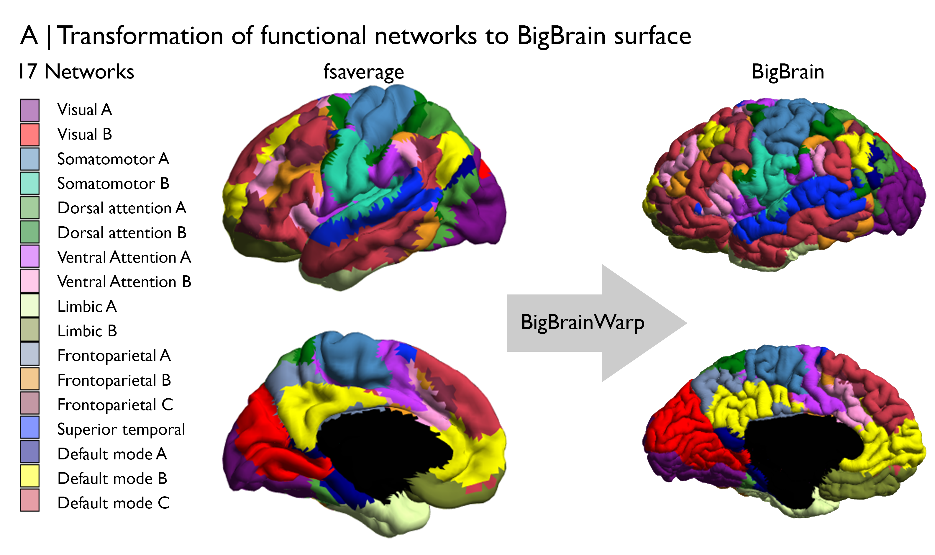
First things first, we should give some forethought to the data and potential transformations necessary for this analysis. Cytoarchitecture can be examined using BigBrain microstructure profiles, which are aligned to BigBrain surfaces. We can define population-average functional communities using the Yeo, Krienen atlas, which is openly available on a variety of standard surfaces and volumes. Given we’re using cytoarchitectural information on the BigBrain surface, we’ll also select a surface version of the Yeo, Krienen atlas. This also conforms with the original creation of the atlas. Specifically, we will use the fsaverage version with 7 functional communities and plan to transform the atlas to the BigBrain surface.
The transformation from fsaverage to the BigBrain surface can be conducted in BigBrainWarp using one line of code. Under the hood, the code involves a multi-modal surface matching informed transformation from fsavearge parcel to BigBrainSym parcels. We’ve already transformed the 7 and 17 Network Yeo, Krienen atlases to BigBrain for you and they can be found in the BigBrainWarp/bigbrain/. Following this interpolation, we should double check visually that the registration is anatomically sound.
bigbrainwarp --in_space fsaverage --out_space bigbrain --wd /local/directory/for/output/ \
        --in_lh /full/path/to/lh.Yeo2011_17Networks_N1000.annot --in_rh /full/path/to/rh.Yeo2011_17Networks_N1000.annot \
        --desc Yeo2011_17Networks_N1000
Check ✔️. We’ve aleady transformed and add some imaging-based atlases, such as these functional networks, to the BigBrainWarp repository. Look for them in the spaces sub-directories.
In this tutorial, we’d like to test the distinguishability of the functional networks based on their cytoarchitecture. To do so, we will load staining intensity profiles from the BigBrainWarp repository and calculate the central moments of each profile. The central moments are an efficient parameterisation of a distribution that have been used with histological data previously to perform observer-independent identification of areal borders (Schleicher, 1999).
% add paths
addpath(genpath(micaopen)) # https://github.com/MICA-MNI/micaopen/
addpath(gifti-master)      # https://www.artefact.tk/software/matlab/gifti/

% load surface
BB = SurfStatAvSurf({[bbwDir '/spaces/bigbrain/gray_left_327680.obj'], ...
        [bbwDir '/spaces/bigbrain/gray_right_327680.obj']});
lh = gifti([bbwDir '/spaces/bigbrain/' parc_name '_lh_bigbrain.label.gii']);
rh = gifti([bbwDir '/spaces/bigbrain/' parc_name '_rh_bigbrain.label.gii']);
parc_bb = [lh.cdata; rh.cdata];
names = [lh.labels.name rh.labels.name];

% load BigBrain profiles and calculate moments
MP = 65536 - reshape(dlmread([bbwDir '/spaces/tpl-bigbrain/tpl-bigbrain_desc-profiles.txt']),[], 50)';
MPmoments = calculate_moments(MP); % caution will take ~60 minutes to run with 10 parallel workers
writetable(table(MPmoments', parc_bb, 'VariableNames', {'mo', 'yeo'}), ...
            [projDir '/output/yeo17_moments.csv'])
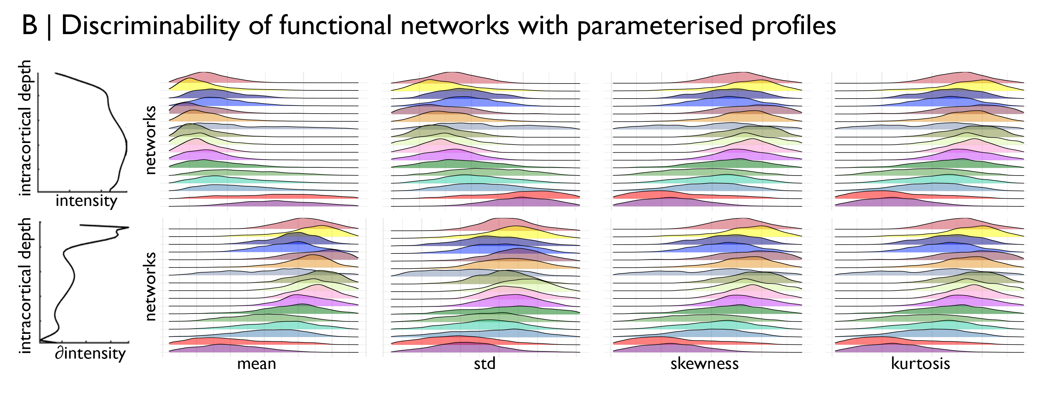
After inspecting the distribution of profile moments across the functional networks, we turn to machine learning to try to functional networks from the staining intensity profiles. First, we divide the data into folds for training and testing, then we export the data to python and run a multi-class classification test
% create 10 folds
folds = 10;
n = floor(6558/folds); % set based vertices in smallest network (DMN-A: 1100)
Xcv_eq = zeros(n*17,size(MPmoments,1),folds);
ycv_eq = zeros(n*17,folds);
for ii = 1:17
    idx = randperm(sum(parc==ii),sum(parc==ii)); % random list of number the length of the network
    idx_net = find(parc==ii); % where is the network in the feature vector
    for cv = 1:folds
        Xcv_eq(((ii-1)*n)+1:(ii*n),:,cv) = MPmoments(:,idx_net(ismember(idx,((cv-1)*n)+1:(cv*n))))';
        ycv_eq(((ii-1)*n)+1:(ii*n),cv) = repmat(ii,n,1);
    end
end
save([projDir '/output/yeo17_moments_bb.mat'], 'Xcv_eq', 'ycv_eq')
# import libraries
import numpy as np
import scipy.io as io
from sklearn.svm import SVC
from sklearn.multiclass import OneVsRestClassifier

# load data
mat = io.loadmat(projDir + "output/yeo17_moments_bb.mat")
X = mat["Xcv_eq"]
ycv = mat["ycv_eq"]
n_classes = ycv.shape[1]
folds = int(X.shape[2])
obs = ycv.shape[0]

# predict in each fold
train_folds = 5
y_pred = np.zeros([obs,train_folds])
for i in range(0,train_folds):
    classifier = OneVsRestClassifier(SVC(kernel='linear'))
    classifier.fit(X[:,:,i], ycv[:,i])
    y_pred[:,i] = classifier.predict(X[:,:,i+train_folds])

io.savemat(projDir + "output/yeo17_moments_pred_ovr.mat", {"y_pred": y_pred})
# back to matlab to create the confusion matrix
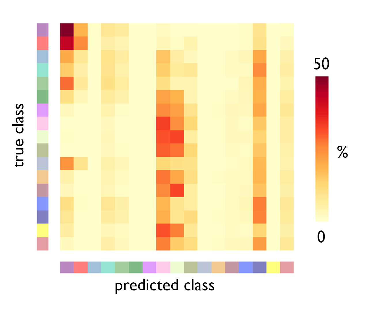
load([projDir '/output/yeo17_moments_pred.mat'])
folds = size(y_pred,2);
confusion_matrix = zeros(7,7,folds);
for cv = 1:folds
for ii = 1:17
for jj = 1:17
confusion_matrix(ii,jj,cv) = sum(ycv_eq(:,cv+5)==ii & y_pred(:,cv)==jj)/sum(ycv_eq(:,cv+5)==ii);
end
end
end
And there we go. Visual networks harbour distinctive cytoarchitecture, reflected by relatively high accuracy and few incorrect predictions. Ventral attention B, limbic and temporoparietal networks are relatively homogenous in cytoarchitecture, related to their restricted spatial distribution. As such, predictive accuracy is moderate but they are also often incorrectly predicted.